Given a set of merged intensities (e.g. downloaded via the “Structure Factors (CIF)” tab on PDB), what is the best practice to convert to amplitude? I see that reciprocalspaceship has this function rs.algorithms.scale_merged_intensities(my_sf_data, "IMEAN", "SIGIMEAN", mean_intensity_method="anisotropic"). Empirically, to what extent do the mean_intensity_method and the associated parameters such as bandwidth or bins matter?
This is a good question that gets to the heart of one of the foundational algorithms in X-ray crystallography. The scale_merged_intensities method is our implementation of the French-Wilson algorithm. This algorithm solves the problem of what to do with the negative intensities that appear in merged datasets due to statistical noise in the data and/or bias in the background estimation. The amplitudes are the square root of the intensities, so you have to be a bit clever to avoid taking the square root of a negative number. The algorithm has two parts. First, it estimates the average intensity in the neighborhood of each reflection. Then it predicts the (strictly positive) structure factor amplitude based on the observed intensity and this estimated average intensity. Your question has to do with the first step.
In most implementations, the neighborhood of each reflection is taken to be a resolution shell. The rs implementation adds the option to define the neighborhood more flexibly as a region in the 3D reciprocal space (mean_intensity_method='anisotropic'). This means two Miller indices with similar resolution might not be in the same “bin” anymore if they are far apart in reciprocal space (ie hkl=30,40,50 and hkl=30,-40,50 would potentially get different mean intensity estimates).
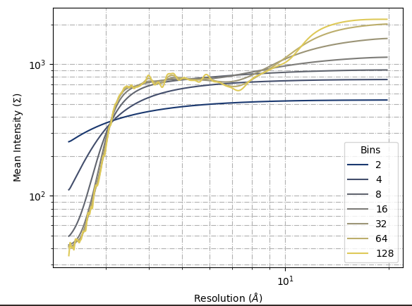
Unless you suspect your data are strongly anisotropic, I would stick with the 'isotropic' option. It’s more consistent with how other packages implement the algorithm. In this case the “bins” argument will determine how rough the mean intensity vs resolution curve will be. You can check this by doing something like this:
import reciprocalspaceship as rs
from reciprocalspaceship.algorithms.scale_merged_intensities import mean_intensity_by_resolution
import seaborn as sns
from matplotlib import pyplot as plt
import numpy as np


bins = [2, 4, 8, 16, 32, 64, 128]
ds = rs.read_cif('9E5R-sf.cif').dropna()
ds = ds.compute_dHKL()
data = []
xkey = r'Resolution ($\AA$)'
ykey = r'Mean Intensity ($\Sigma$)'
for b in bins:
    sigma = mean_intensity_by_resolution(ds.IMEAN, ds.dHKL, b)
    data.append(rs.DataSet({
        xkey : ds.dHKL,
        ykey : sigma,
        'Bins' : np.ones_like(sigma, dtype='int') * b,
    }))
data = rs.concat(data, check_isomorphous=False)
data['Bins'] = data['Bins'].astype(str)
sns.lineplot(data, x=xkey, y=ykey, hue='Bins', palette='cividis')
plt.loglog()
plt.grid(which='both', axis='both', ls='-.')
plt.show()
If you still want to use the “anisotropic” mode, the advice I can give you is that the bandwidth is in Miller index units. There appears to be some reasonable range between 0.25 and 4.0. Much larger than that and the mean intensity estimates collapse to be the same for all reflections.
import reciprocalspaceship as rs
from reciprocalspaceship.algorithms.scale_merged_intensities import mean_intensity_by_resolution,mean_intensity_by_miller_index
import seaborn as sns
from matplotlib import pyplot as plt
import numpy as np
import matplotlib.animation as animation


bw = [0.25, 0.5, 1., 2., 4., 8., 16., 32.]
ds = rs.read_cif('9E5R-sf.cif').dropna()
ds = ds.compute_dHKL()
data = []
xkey = r'Resolution ($\AA$)'
ykey = r'Mean Intensity ($\Sigma$)'
for b in bw:
    sigma = mean_intensity_by_miller_index(ds.IMEAN, ds.get_hkls(), b)
    data.append(rs.DataSet({
        xkey : ds.dHKL,
        ykey : sigma,
        'Bandwidth' : np.ones_like(sigma, dtype='int') * b,
    }))
data = rs.concat(data, check_isomorphous=False)


fig, ax = plt.subplots()
ax.set_xscale('log')
ax.set_yscale('log')
ax.set_xlabel(xkey)
ax.set_ylabel(ykey)

data = data.sort_values(xkey)
b = 1.0
title = ax.set_title(f"Badwidth = {b}")
idx = (data['Bandwidth'] == b)
ds = data[idx]
line, = ax.plot(ds[xkey], ds[ykey], color='k', alpha=0.3)
xlim = ax.get_xlim()
ylim = ax.get_ylim()
plt.grid(which='both', axis='both', ls='-.')


def animate(i):
    b = bw[i]
    title.set_text(f"Badwidth = {b}")
    idx = (data['Bandwidth'] == b)
    ds = data[idx]
    line.set_ydata(ds[ykey])
    ax.set_xlim(xlim)
    ax.set_ylim(ylim)
    return line,


ani = animation.FuncAnimation(
    fig, animate, repeat=True, frames=len(bw), interval=500
)
writer = animation.PillowWriter(fps=0.5, bitrate=1800)
ani.save('line.gif', writer=writer)

plt.show()
Good question! Hope this helps. Happy to follow up with more info if needed.
2 Likes